A downloadable version of this activity is available in the following format:
We often want to find out something about an entire population, but are unable to collect information about the whole population. We need to rely on the information we collect from only a part of the population (a sample) to tell us what we want to know about the whole population. (In other words, the sample is a small ‘snapshot’ of the bigger picture.) For example, statisticians calculate the monthly unemployment rate in Canada by collecting data from a sample of all working-age people. Surveying the entire population would be too costly and time-consuming.
In order to get information on the whole population, we need to know how to interpret the sample. Before looking at samples, let’s start by considering a population for which we can see the big picture. The data table below gives the heights in centimetres of apopulation of 100 15-year-olds.
| 165 | 161 | 170 | 182 | 176 | 185 | 180 | 155 | 154 | 166 |
| 165 | 152 | 174 | 167 | 165 | 171 | 172 | 150 | 181 | 165 |
| 166 | 161 | 174 | 158 | 166 | 168 | 164 | 150 | 155 | 170 |
| 168 | 144 | 164 | 154 | 177 | 173 | 178 | 158 | 165 | 175 |
| 180 | 174 | 152 | 167 | 148 | 175 | 153 | 162 | 180 | 175 |
| 157 | 172 | 155 | 140 | 147 | 160 | 152 | 166 | 168 | 158 |
| 153 | 165 | 160 | 143 | 166 | 167 | 167 | 163 | 158 | 160 |
| 150 | 157 | 172 | 167 | 184 | 172 | 165 | 159 | 158 | 177 |
| 179 | 174 | 156 | 178 | 165 | 179 | 174 | 148 | 175 | 166 |
| 157 | 159 | 163 | 165 | 162 | 153 | 145 | 170 | 176 | 180 |
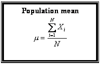
| The mean of the population is 164.7 | The standard deviation is 10.2 |


N = size of the population
1. To begin, be sure you understand how to calculate the mean and the standard deviation of a population. Describe each process in words.
2. In Handout 1, look at “Histogram 1: Original data.”
a. Draw a vertical line to indicate the mean on the graph.
b. If possible, determine the median and mode from the histogram.
c. Draw the frequency polygon. Describe its shape.
d. Comment on the variation evident in the graph.
This is the big picture of our population. However, if we could only collect information from a sample, do you think the sample would really reflect the population? Would different samples all have a histogram that looks the same as that of the population? Would they have the same mean?
3. As a class, take a relatively large number of different samples (e.g., 100) from the list of heights of our population. Then look for connections between the means and standard deviations of the samples and those of the whole population.
a. Create a random sample of five heights. Describe how you ensured that the sample was random. Record the heights that you randomly selected.
b. Calculate the mean of your sample (correct to one decimal place).
c. Repeat until you have pulled your share of the class’s 100 samples. (The teacher will assign your share.) Record each sample’s mean.
4. a. Using the 100 sample means collected from the class, complete the frequency Table below.
(Note: The table uses intervals of one unit. For example, 145 includes all sample mean values equal to or greater than 145 up to but not including 146. Therefore, 145.3 is included in the interval 145 to 146, which you would indicate on the frequency table as 145.)
Sample means for n= 5
| Class | Tally | Frequency | Class | Tally | Frequency | |
| 145 | 163 | |||||
| 146 | 164 | |||||
| 147 | 165 | |||||
| 148 | 166 | |||||
| 149 | 167 | |||||
| 150 | 168 | |||||
| 151 | 169 | |||||
| 152 | 170 | |||||
| 153 | 171 | |||||
| 154 | 172 | |||||
| 155 | 173 | |||||
| 156 | 174 | |||||
| 157 | 175 | |||||
| 158 | 176 | |||||
| 159 | 177 | |||||
| 160 | 178 | |||||
| 161 | 179 | |||||
| 162 | 180 |
b. Sketch the histogram and frequency polygon on Grid 2 of Handout 1.
c. Compare the shape of this frequency polygon with that of the original data.
d. Calculate and record the mean and standard deviation of the sample means.
5. There are other ways to generate samples of the original data. Fathom statistical software was used to generate 100 different random samples of 20 students from the original population of 100 students (See Appendix A). The sample means were calculated and the frequency table is given below.
| The mean of the sample means is 164.5. The standard deviation of the sample means is 2.2. |
|
Sketch the histogram and frequency polygon for 100 samples of 20 heights on Grid 3 of Handout 1.
6. Consider the three graphs on Handout 1. Comment on each and suggest an explanation for
a. the shape of the histograms of the sample means,
b. the mean of the sample means for different sample sizes
c. the standard deviation of the sample means as the sample size increases. What is the approximate ratio of the standard deviation for 20 heights compared with the standard deviation for 5 heights?
7. Describe in words what you would expect if 100 different samples of 40 heights were chosen? What would you predict about
a. the shape of the histogram of the sample means?
b. the mean of the sample means?
c. the standard deviation of the sample means?
Clearly, the variation is related to sample size. Does it also depend on the number of samples taken?
8. See Handout 2 —Different numbers of samples and different sample sizes. The same height data were used to generate 100, 500 and 1,000 samples for n = 30 (graphs 2, 3 and 4) and 500 and 1,000 samples for n = 50 (graphs 5 and 6).
Examine the graphs and the recorded information. Comment on
a. the shapes,
b. the means of the sample means, and
c. the standard deviations of the sample means.
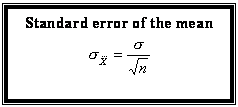
9. We used the calculation for standard deviation to get a measure of the variation in the sample means. This measure of variation is commonly referred to as the standard error of the mean, ![]() .According to the formula below, it depends only on the standard deviation in the population,
.According to the formula below, it depends only on the standard deviation in the population, ![]() , and the sample size, n.
, and the sample size, n.

Use the formula to calculate the standard error of the mean for samples of 30 heights and 50 heights. How do these values compare with calculations of standard deviation in the table?
Conclusion
We now have the following:
- a distribution of sample means
- a connection between the mean of the sample means and the population mean
- a connection between the standard deviation of the population mean and the standard error of the mean
Contributed by Anna Spanik, Math teacher, Halifax West High School, Nova Scotia.

